Rip Van Winkle's Code

Problem Name: Rip Van Winkle’s Code
UVa ID: 12436
LightOJ ID: 1411
Keywords: segment tree, lazy propagation

Today we’ll take a look at a problem from this year’s ACM ICPC World Finals Warmup contest, and which can be solved with the help of segment trees. It will give us an opportunity to contemplate some more of the nice subtleties that often come into play in this type of problem.

We’re asked to consider an array of 64–bit integers. The size of this array is fixed at 250,001 positions (index 0 is left unused, so we have to focus only on positions 1–250,000) and it is initially filled with zeroes. Three types of operations can modify this array:

• Operation A takes two integers, let’s call them \(i\) and \(j\), and adds 1 to position \(i\) of the array, 2 to position \(i+1\), 3 to \(i+2\) and so on. In other words, it increases the values in the range \([i:j]\) of the array according to the sequence \(1, 2, 3, \ldots, (j-i+1)\) from left to right.
• Operation B is similar to A, but it applies the additions in a right–to–left fashion (it adds 1 to position \(j\), 2 to position \(j-1\) and so on).
• Operation C is simpler. It also takes two integers that describe a range, but it receives an extra argument; an integer \(x\). All positions in the range \([i:j]\) of the array are then set to \(x\).

Finally, we have a fourth operation S which doesn’t alter the array, it must simply report the sum of all positions in a given range \([i:j]\) of the array.

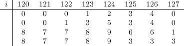
Let’s quickly illustrate these operations with an example. We’ll consider the arbitrary range \([120:127]\) of the array. At first, this range looks like this:

Now, let’s say that we receive the following commands to execute in order:

• A 123 126
• A 122 124
• B 120 127
• C 125 127 3

Then the changes inside the data array would look as follows:

Okay, now that we’re a bit more familiar with the problem, let’s give it some thought. As I mentioned in the beginning, we’ll base our approach on the powerful segment tree data structure. With this in mind, it would seem that implementing operations C and S could be fairly straightforward. However, operations A and B are somewhat tricky. They modify a range of values, but each position in that range is modified differently. We should, however, try to implement those commands in a way that involves just one update on the tree (with complexity \(O(\log{N})\)), otherwise our code wouldn’t be too efficient.

Let’s start by visualising our segment tree for the small range we chose in our example. We’ll start with the basics, just storing in each node of the tree the total sum of the corresponding range. We’ll extend this tree gradually as we see fit.

This tree represents the range \([120:127]\) of a fresh array, so it’s filled with zeroes. The first row in each node contains its index and range, while the second row contains the sum of all positions in the corresponding segment in the array. Notice that the nodes of this tree have been indexed using the numbers \(1, 2, \ldots, 15\), but in reality these nodes would receive different indices —node 1 would be for the real root of the tree, which covers the range \([1:250,000]\), node 2 would be its left node, and so on. Numbers 1 to 15 are used here just to simplify things a bit in the following examples, but keep in mind that they would not be the real indices in the segment tree for the whole array.

Alright, let’s consider our first query: A 123 126. How would the tree be affected by this command? We could produce something that looks like this at first:

By looking at this tree, a few things are brought to our attention. One is that the value of each affected node is increased according to a sequence of consecutive integers, but the sequence is of course different for each node. For example, node 6 was increased by 5, which is the result of \(2+3\). For that node, the sequence applied to increase the values in the range \([124:125]\) started with 2, and its length is 2 of course. Another important thing that this graph seems to “shout” at us, is that we must devise a strategy for the propagation of this update. The situation is pretty evident in nodes 12 and 13. How can we tag these nodes so they are properly updated down the road?

But let’s pause for a second and think on the situation of sequences of consecutive integers that start with an arbitrary number. We’ll generalise and consider a node that represents a segment of length \(k\). The contents of the node (the sum of all values in its range) will be denoted \(S\). When we receive an A operation that affects this node, we have to change its contents according to a sum of the form:

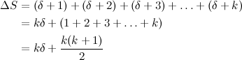
Where \(\delta\) represents the distance of each element in the base sequence \(1, 2, 3, \ldots, k\) to the corresponding element in the actual sequence applied to the node, which could start with any positive integer. To illustrate this, we can see in the graph above that, for node 11, \(k=1, \delta=0\); for node 6, \(k=2, \delta=1\); and for node 14, \(k=1, \delta=3\).

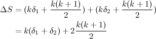
This method of representing the A operation has also the benefit of working out nicely when we accumulate the results from more than one command of this type for the same node. The value of \(k\) remains the same in each node, so the only thing that could change is \(\delta\). Let’s say that a certain node receives two A operations, one after the other, with two values \(\delta_1\) and \(\delta_2\). This would result in the following:

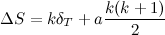
In general, if a node receives \(a\) operations of type A, with a total \(\delta_T\) —the result of adding \(\delta_1, \delta_2, \ldots, \delta_a\)— then all these changes can be represented by the expression:

And what about the B operation? Well, if you think about it for a minute, it should be easy to notice that it works very similarly to an A operation. The difference is that the \(\delta\) values are calculated differently (right to left) and that, in order to facilitate the calculation of \(\delta\) values for children nodes, it would be convenient to keep track of the number of B operations with a different variable (let’s call it \(b\)).

Putting all of this together, we can now extend each node of the segment tree with three additional values: \(a\) (the number of A operations to propagate), \(b\) (the number of B operations to propagate), and \(\delta\) (the sum of all \(\delta\) values from either A or B operations). Let’s see how our tree looks like now:

What is nice about this approach is that, given that every node is implicitly associated with a given range of the array, it is easy to determine the values of \(k\) and \(\delta\) in each node (and their children) for every A and B operation. And calculating the new \(S\) from \(a\), \(b\) and \(\delta\) is even easier.

Let’s quickly review how the tree changes with the rest of the operations we used in our original example. After the operation A 122 124 we would have:

And after B 120 127:

Note that, as I mentioned in the analysis of Ahoy, Pirates!, there are some things that happen behind the curtains while propagating updates down the tree. For example, when the second A operation is issued, the tree is traversed down to node number 12, and in the process node 6 and its children are visited, and that’s when node 13 is updated so its \(S\) value becomes 3, while \(a, b, \delta\) are cleared.

Now we have only one operation left to implement: C. We could try to implement it using the \(\delta\) field we have already defined, but that would represent some difficulties when several commands are stacked for future lazy propagation. Consider for example a C command followed by an A operation and vice–versa. To avoid these issues, and for commodity, we’ll simply create a couple of new fields: one boolean field \(c\) that represents whether a C operation is pending or not, and a field \(x\), which is simply the argument for the corresponding C operation.

Let’s see this new extended tree, and how it would change after the command C 125 127 3:

Once again, a few nodes have changed purely as a side–effect of traversing the tree (e.g. nodes 2, 4 and 5). It’s also worth mentioning that once a C operation is passed on to a child node for lazy propagation, the \(a\), \(b\) and \(\delta\) fields of the child are cleared, because the C operation overrides any previous commands. This can be seen, for example, in nodes 14 and 15. However, A and B do not override previous commands.

---

Okay, we have reached the end of this analysis. I’d like to end by commenting on something that I realised while working on this problem, which is that I’ve developed a special appreciation for algorithm problems related to segment trees, because they typically require a little bit of… I guess you could call it “inspiration”, to nail the right representation of the relevant data and to imagine how every operation should work and be propagated through the tree. Not only that, these problems also demand a lot of attention to detail in the implementation, because with so many subtle things to keep track of, it’s easy to make a mistake somewhere.

How nice it is that we all have the opportunity to sharpen our skills by working on fun problems like this one :).