A Dangerous Maze (II)

Problem Name: A Dangerous Maze (II)
LightOJ ID: 1395
UVa ID: 12411
Keywords: probability, expected value

You are inside a maze, in front of a series of doors. By choosing a door, you follow a path, taking a certain amount of time, and at its end you find yourself either out of the maze, or back at the beginning. The question is, if the probability for choosing any given path is the same for all doors, then what is the expected amount of time to get out if the maze (if it’s at all possible)?

However, there’s an interesting twist: you also remember the last \(K\) decisions you made, and if you have previously chosen a door that takes you back to the beginning, you won’t select it again, as long as it remains one of your last \(K\) decisions.

I found the concept behind this problem very interesting, and at first I tried to come up with some sort of dynamic programming solution. However, after some consideration, it became clear that such an approach would be infeasible due to the problem constraints (the number of doors \(n\) can be 100, and \(K\) can be any number between 0 and \(n\)), and the intricate relations formed when you consider your K–sized memory.

So I tried the pure math way… armed with a pencil and a stack of paper, I filled many pages with equations and drawings to help me model the problem conveniently, making some mistakes along the way, correcting them, trying to find some kind of pattern until I could identify something that could let me formulate a conjecture that I could then translate into code. In this post I’ll try to summarise my findings.

First of all, let’s split the doors into two sets, and label them as follows:

Where \(a_i\) is the time for the ith door that takes you out of the maze, and \(b_i\) is the time for the ith door that leads you back to where you started. The total number of “positive” doors (the ones that lead you out) is denoted \(p\), and the total number of “negative” doors (the ones that take you back to the beginning) is \(q\). Notice that \(n=p+q\).

Now, let’s define \(E\) as follows:

\(E(S)\)

The expected amount of time to get out of the maze, after having visited the sequence of doors \(S\).

The sequence (ordered list) given as argument to the \(E\) function is important because it represents your “memory”.

When you’re just starting your journey, you haven’t visited any doors, so the value of \(E\) would look like this:

In other words, \(E\) is defined recursively, based on the fact that whenever you choose one of the \(b\) doors, you are back at the beginning, but having added your last decision to your sequence (note the use of parenthesis as notation for the sequences).

Let’s add a few more definitions, in order to simplify the expressions that come a little further below:

\(\hat{E}_i\)

The sum of all possible \(E(S)\), where \(S\) has exactly \(i\) elements.

With this, let’s reformulate \(E(())\), and see what happens when \(K=0\):

The equation [2] is the answer for the case where \(K=0\), meaning you can’t remember any previous decisions (which is, by the way, the same situation as in the first A Dangerous Maze problem, LightOJ ID 1027).

Things start to get interesting when you consider \(K > 0\):

Equation [3] requires the most attention, but it’s simply the result of thinking what is the result of adding \(E(\,(b_u)\,)\) for all possible values of \(b_u\).

The same reasoning can be used for \(K=2\) and \(K=3\), but doing the actual calculations for \(\hat{E}_2\) and so on becomes increasingly difficult. You can try to deduce all of this for yourself, but suffice to say that the results for \(E\) with the first values of \(K\) are the following:

Can you see the pattern? (Also, do you see how I managed to fill pages upon pages with my conjectures and wrong turns?)

All in all, a very nice problem, with some interesting mathematics behind it. I still don’t know if there’s a shorter way to deduce the general formula (maybe using some number or probability theory I’m not aware of), instead of just using conjectures… If you have any ideas, let me know :).

Marriage Ceremonies

Problem Name: Marriage Ceremonies
LightOJ ID: 1011
Keywords: dynamic programming, bitmask calculations

Given a matrix of values for all possible matches between \(N\) men with \(N\) women, we need to find out the maximum possible value after matching all people. It is, as one would suspect, completely reasonable to solve it using D.P. What makes this problem interesting is that the D.P. function depend on sets of values, rather than just one or two scalar variables, as is usually the case.

Consider for example the following definition:

\(f(i, S)\)

The maximum result value after matching \(i\) men with the set of women \(S\), where \(S\) has exactly \(i\) elements.

To calculate \(f\), first consider the basic case: where \(i=1\). In this case:

where \(p(i, j)\) is the priority between the ith male and the jth female, as given in the input.

Then, for \(f(i, S)\) where \(i > 1\), we have:

In other words, for every new man (the ith man) that we want to match with someone, we try adding his priority against every woman (\(S_j\)) and the maximum from marrying all men up to \(i-1\) with the set of all women except \(S_j\). For example, to calculate \(f(3, \{1, 2, 3\})\), we require the values of \(f(2, \{2, 3\})\), \(f(2, \{1, 3\})\) and \(f(2, \{1, 2\})\).

All of this is good in abstract, but how to represent the sets efficiently? This is where the bitmask concept kicks in. You should be familiar with binary representation of integers, and with bitwise operations. The idea is to use a single integer to represent all possible sets of values, which is feasible in this case because \(N\) is at most 16, so the space required for our D.P. structure would be \(16 \times 2^{16}\).

Now, although a recursive implementation may be easier to write and understand, let’s try writing an iterative version of our D.P. function. Consider the following C++ fragment:

typedef unsigned int u32;

// dp[i][j] will contain the maximum priority of marrying i men with the set
// of women defined by the bitset j
int dp[MAXN + 1][1 << MAXN];

void run_dp()
{
    for (int i = 1; i <= N; ++i)
        dp[1][1 << (i - 1)] = pri[1][i];

    u32 top = 1 << N;

    for (int i = 2; i <= N; ++i) {
        u32 b = (1 << i) - 1;

        for (u32 j = b; j < top; j = next_popcount(j)) {
            b = j;  // women still untested
            int max = 0;

            while (b != 0) {
                u32 w = b & -b;  // bit of the next woman to consider
                int idx = pos[w];

                int curr = pri[i][idx] + dp[i - 1][j & ~w];
                if (curr > max) max = curr;

                b &= ~w;  // w has been tested, remove it
            }

            dp[i][j] = max;
        }
    }
}

In lines 9-10, the first row of values is filled as described above (pri is the matrix of values from the input). Note that the set \(\{1\}\) is represented as an integer with the least significant bit set, the set \(\{2\}\) is represented by an integer with the second least significant bit set, and so on.

Then all the other rows are filled in the loop at line 14. Note how all possible sets of exactly \(i\) women are represented by the \(j\) variable. It is set initially to the value calculated on line 15, which uses simple bitwise manipulations to obtain an integer with the first \(i\) bits set.

A few other relevant details: first, a function called next_popcount is used, and it must return the next integer, strictly greater than its argument, that has the same number of bits set (that number is sometimes called the “popcount”). A concise implementation of this function, courtesy of hakmem 175, is this:

u32 next_popcount(u32 n)
{
    u32 c = (n & -n);
    u32 r = n+c;
    return (((r ^ n) >> 2) / c) | r;
}

Second, the pos array is simply an auxiliary variable to easily map single-bit bitmasks to the positions they represent. For example pos[1 << 0] is 1, pos[1 << 1] is 2, and so on.

Finally, have you noticed the curious expression of the form (x & -x) that is used a couple of times? It simply produces an integer where the only bit set is the least significant bit set in the x variable. That’s an interesting trick that is useful to remember.

A final note on using bitmask calculations for D.P. programs; sometimes writing a recursive implementation may not only be easier to write, it could also run much faster. Sometimes filling the whole D.P. structure (which requires calculations for every possible combination of bits) is not really necessary, so writing a recursive function where only the required values are calculated can be order(s) of magnitude faster. This is the case, for example, in the problem Brush (IV) (LightOJ ID 1018).

Explosion

Problem Name: Explosion
UVa ID: 11861
LightOJ ID: 1407
Keywords: 2sat, graph, strongly connected components, backtracking

This is an interesting 2-SAT problem. As most 2-satisfiability problems, it can be solved using a graph that represents the corresponding CNF formula, and working on its strongly connected components.

However, the interesting part comes in the “council opinions” given in the input, which represent constraints with 3 variables. Since \(k\) is at most 5, a little bit of brute force should work.

I tried this at first, and wrote a brute force solution that tried all \(3^k\) options (reconstructing the S.C.C.s for each alternative) and, of course, it was very slow…

What is required is a little bit of pruning. This is where the “back-tracking” part comes up. If \(k=0\), then running the standard 2SAT algorithm one time is sufficient. But if \(k > 0\), you can start by checking the 2SAT on the original graph (without any council options), and if its value is false (can’t be satisfied), then you can give your answer and you’re finished. Otherwise, start testing with all options from the first council member, and only go deeper in the tree of options if the 2SAT algorithm up to that point returns true.

The idea is to add constraints from the council members one at a time, and if at some point the 2SAT graph can’t be satisfied, then it’s not necessary to go through any of the remaining council members for that branch.

This reduces the number of steps drastically, and is enough for an AC.

Winning Streak

Problem Name: Winning Streak
UVa ID: 11176
Keywords: dynamic programming, probability, expected value

This is a very nice problem that involves probability and dynamic programming. What I find particularly nice about it is that formulating the D.P. structure requires, I think, a little creativity.

First, it’s necessary to understand how the expected value is calculated, and how are the probabilities of separate events combined to produce the probability that all events occur.

With that out of the way, and after some time pondering on how to model this problem for a D.P. solution, we could initially define the relation \(f(i, j)\) as follows:

\(f(i, j)\)

The probability of having a winning streak of exactly \(j\), after \(i\) games.

However, it is more convenient to define it slightly different, for reasons that will become apparent in the reasoning below:

\(f(i, j)\)

The probability of having a winning streak of \(j\) or less, after \(i\) games.

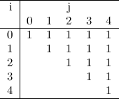
For example, \(f(5, 3)\) would be the probability of having a winning streak of 0, 1, 2 or 3 after 5 consecutive games. Then we can begin to see how our D.P. data structure will be filled. First of all, for all pairs \((i, j)\) where \(j \geq i\), it’s easy to see that the probability is 1:

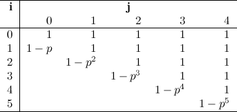
Now, when \(j = i-1\), the value of \(f(i,j)\) will be \((1 - p^i)\), where \(p\) is the probability of winning a game. This is because the only way to have a winning streak of \(i\) in \(i\) games is winning them all in a row (hence the \(p^i\)), and that is the only case that need to be excluded from \(f(i, i - 1)\).

We have now:

For the remaining positions (\(j < i-1\)), we need to figure a way to calculate their values, relating it to what we already have. Let’s compare the meaning of \(f(i, j)\) and \(f(i-1, j)\).

When we think about \(f(i-1, j)\), we recognise that it corresponds to the probability of the sequences of games:

Where \(G_k\) for all \(k\) between 1 and \(i-1\) is either W or L, and where there are at most \(j\) consecutive W’s. Similarly, \(f(i, j)\) is the sequence:

Where there are also at most \(j\) consecutive W’s. Let’s consider what is happening with \(G_i\). It could be L, in which case nothing changes, because it doesn’t create any winning streak bigger than \(j\). Or it could be W, and in that case, we need to remove those cases where it does create a winning streak of \(j+1\).

Given that we can be sure that in the sequence up to \(G_{i-1}\) there are at most \(j\) consecutive W’s, then the only way for \(G_i\) to create a winning streak of \(j+1\) is this:

And so, we reach to the formula for our remaining positions (where \(j < i-1\)):

To get our answer we just need to iterate over the nth row of our data structure, and use the fact that \(f(n, j) - f(n, j-1)\) is the probability of having a winning streak of exactly \(j\) in \(n\) games.

Our final implementation in code then could look something like this:

// dp[i][j] will have the probability of having a maximum winning streak of
// j in i consecutive games
double dp[MAXN + 1][MAXN + 1];

// pp[i] will have p^i
double pp[MAXN + 1];

int n;       // from the input, the number of consecutive games
double p;    // from the input, the probability of winning 1 game
double ans;

void run_dp()
{
    pp[0] = 1.0;
    for (int i = 1; i <= n; ++i) pp[i] = pp[i - 1] * p;

    for (int j = 0; j <= n; ++j)
        dp[0][j] = 1.0;

    for (int i = 1; i <= n; ++i)
        for (int j = 0; j <= n; ++j) {
            dp[i][j] = dp[i-1][j];

            if (j == i - 1)
                dp[i][j] -= pp[i];
            else if (j < i - 1)
                dp[i][j] -= dp[i - j - 2][j] * (1-p) * pp[j+1];
        }

    ans = 0.0;
    for (int j = 1; j <= n; ++j)
        ans += j * (dp[n][j] - dp[n][j - 1]);
}

Not the Best

Problem Title: Not the Best
LightOJ ID: 1099
Keywords: dijkstra, single source shortest path, graph

This is a graph problem where, instead of finding the shortest path from point A to point B (which is the usual setup in this type of problems), it asks for the second best path, which is a path that is strictly longer than the shortest path(s), possibly visiting any edge or vertex more than once.

This can be solved by modifying a traditional Dijkstra algorithm, although you need to do it carefully. The beauty of this problem is that it puts your knowledge of this algorithm to the test. If you don’t have a deep understanding on how this algorithm works, coming up with a solution from this angle might not be very easy.

Anyway, the solution I came up with basically involves keeping track of 2 distances for each vertex: the best distances from the source, and, of course, the second best distances from the source. To illustrate the idea, I’ll use the following pseudo-code for Dijkstra’s algorithm, based on a snippet from Wikipedia, slightly modified to illustrate an implementation based on a priority queue:

function Dijkstra(Graph, source):
    for each vertex v in Graph:
        dist[v] := infinity ;
        vis[v]  := false ;     // flag to tell if a vertex has been visited
    end for ;
    dist[source] := 0 ;

    Q := a priority queue of tuples (d,v) ;
    push (0,source) to Q ;

    while Q is not empty:
        u := second element of the tuple from the front of Q ;
        pop front element from Q ;

        if vis[u]:
            continue ;
        end if ;
        vis[u] := true ;

        for each neighbor v of u:
            alt := dist[u] + dist_between(u, v) ;
            if alt < dist[v]:
                dist[v] := alt ;
                push (dist[v], v) to Q ;
            end if ;
        end for ;
    end while ;
    return dist[] ;
end Dijkstra.

Straightforward enough. A couple of things to notice: The tuples that are stored in Q have two elements, the first one represents a distance, and the second a vertex number. These tuples are sorted inside the queue according to their contents, first by the first element, and then by their second element (much like how C++ STL pairs behave).

Make sure that you understand what every step of this algorithm does, otherwise now would be a good time to read and think a little more about it.

Not let’s see the modifications that could be used to solve this problem:

// Second best (shortest) paths from single source
function Dijkstra2(Graph, source):
    for each vertex v in Graph:
        // Two dimensions to represent the two best distances
        dist[1][v] := infinity ;
        dist[2][v] := infinity ;
        vis[1][v]  := false ;
        vis[2][v]  := false ;
    end for ;
    dist[1][source] := 0 ;

    Q := a priority queue of tuples (t,d,v) ;
    push (1, 0, source) to Q ;

    while Q is not empty:
        t := first element of the tuple from the front of Q ;
        u := third element of the tuple from the front of Q ;
        pop front element from Q ;

        if vis[t][u]:
            continue ;
        end if ;
        vis[t][u] := true ;

        for each neighbor v of u:
            alt := dist[t][u] + dist_between(u, v) ;
            if alt < dist[1][v]:
                dist[2][v] := dist[1][v] ;
                push (2, dist[2][v], v) to Q ;

                dist[1][v] := alt ;
                push (1, dist[1][v], v) to Q ;
            else if alt > dist[1][v] and alt < dist[2][v]:
                dist[2][v] := alt ;
                push (2, dist[2][v], v) to Q ;
            end if ;
        end for ;
    end while ;
    return dist[2][] ;
end Dijkstra2.

As you can see, the idea is pretty simple, but the changes require attention to important details.

First of all, notice that the dist and vis arrays are two-dimensional arrays now, and the first index could be 1 or 2, representing the best or second-best path respectively.

Also, at line 12, the tuples that we store in Q have three elements now, where the first one is an integer to represent the type of tuple (1 or 2, as described for the dist and vis arrays).

Finally, notice how the decisions on what to push to the queue are affected. If a new best distance to a vertex is found, then the previous one is bumped as the new second-best distance (lines 28-29).

Also, if the alternative distance is strictly larger than the best path, but is better than the second-best, then it needs to be used (line 33).