Saturday, 29 September 2012

Jogging Trails

Problem Name: Jogging Trails
UVa ID: 10296
LightOJ ID: 1086
Keywords: graph, dynamic programming, eulerian cycle, floyd-warshall, bitmask calculations, chinese postman

In the world of competitive programming, it is very common to come across problems that place the focus on just one or two main algorithmic concepts, such that you can more or less solve them by simply following a “standard” recipe, or by doing a few simple variations over the classic algorithms. However, not every problem is like that.

There are problems that involve several different concepts, and their algorithmic elements intertwine in interesting and elegant ways to create a new type of challenge. A challenge that provides great satisfaction and a powerful sense of fulfillment once you find out a valid way to rearrange and mix the ingredients from different recipes to create your own solution. Moreover, from my own limited experience observing the work of some of the greatest competitive programmers on the planet, it is my belief that perhaps the main difference between them (the really, really good algorithm problem solvers), and the average programmers —beyond the obvious things, like the amount of experience and knowledge—, is their deep understanding of the “recipes” and their creativity to mix them in order to solve a new complex problem.

Jogging Trails, the problem I’ll talk about here, is a relatively “simple” problem, but it’s a very nice example of this type of beautiful “intertwining” of different concepts. It’s easy to summarise the problem like this: you receive a weighted, undirected and connected graph; you have to find the “cost” of the shortest route that starts and ends on the same vertex after visiting every edge at least once. This is also known as the Chinese postman problem, or the route inspection problem.

There are many interesting things to talk about in this problem, so we’ll approach them gradually. Let’s start with an example to help us illustrate our ideas down the road. Consider the following graph:

Okay, first things first. Try to manually find the solution for this example. Finding it quickly is not very easy. One of the first things you’ll probably notice is that it’s tricky to find a route that starts and ends on the same node, after having visited each edge exactly once. In fact, it’s impossible.

This is where the first interesting algorithmic idea comes to play, and it is that of an Eulerian cycle or circuit. It simply refers to a cycle inside a graph that visits each edge exactly once. What is useful to remember is this (quoting from Wikipedia):

An undirected graph has an Eulerian cycle if and only if every vertex has even degree, and all of its vertices with nonzero degree belong to a single connected component.

In other words, assuming you have a connected graph (like in our case), count the number of edges connected to each node and if every node has an even number of them, then you absolutely can do a tour that starts and ends on the same place, and visits all edges exactly once. This means that if our example showed that property (every node had an even degree), then we would not have to do anything special, the answer would just be the sum of weights of all edges. Simple, right? Remember that we don’t need to calculate the path itself, just its cost.

However, we aren’t that lucky in our example. We have five nodes, and four of them have an odd degree. What this implies is that whatever shortest path there might exist in there, it must visit some edges more than once, there’s no other way around it. The question is, obviously, which edges will we have to visit twice or more? Actually, we don’t really need to know which edges, just how much additional cost will they represent for our final answer.

At this point, it could be useful to apply a general strategy that is usually seen in graph–related problems. If you know of a certain algorithm or idea that can help you but it can’t be applied to your graph directly, try modifying your graph until it does! This is a common technique used, for example, when you want to calculate things like the max flow in a network and so you invent “dummy” nodes and edges in order to apply the algorithm properly.

In this case, what if we think about “dummy” edges that can turn all nodes into even–degree nodes? Something like this:

There are many possible ways in which these fake edges could be created to make this graph favourable for finding an Eulerian cycle. We could, for example, connect nodes \((2, 3)\) and \((1, 4)\), or we could do \((2, 1)\) and \((3, 4)\), and for each of these connections there are many ways to do it as well. For instance, for the fake edge \((2, 3)\) there are many ways to go from 2 to 3, like going directly (with a cost of 25), or going through node 1 (with a cost of 23). It is important to keep in mind that the fake edges are just something to help us model the graph as something where you can actually find an Eulerian tour, but they just represent paths that exist over the real edges.

In any case, what we’re interested in is a combination of fake edges that provide the minimal additional cost. So we arrive to the second algorithmic idea to be applied in this problem. In order to try the different available combinations that can form our fake edges, it is in our best interest to find out the shortest paths between all pairs of nodes, and since the number of nodes in the graph is very low (\(n \leq 15\)), the Floyd-Warshall algorithm fits the bill perfectly.

After this step, we would end up with the following information:

A little examination should reveal that the best possible combination of fake edges among the nodes \((1, 2, 3, 4)\) would be from the shortest paths between \((1, 2)\) and \((3, 4)\). Our extended graph would then look like this:

Try finding the solution now. Doing an Eulerian tour is now a breeze, and it is pretty evident that the edges that have to be visited twice are \((2, 1)\), \((4, 5)\) and \((3, 5)\). The final answer for this example is 109, the sum of all edges in this extended graph.

We are getting close, but we still haven’t figured out just exactly how are we going to find the best combination of fake edges. This is where the third and final algorithmic concept comes in: dynamic programming, with a little bit of bitwise manipulations.

Again, because the number of nodes is small, it is feasible to formulate the following D.P. relation:

\(f(S)\)
The minimum cost of connecting pairs of nodes among the set \(S\) (represented as a bitmask in code).

This relation is very simple: the base case is an empty set of nodes, which has a cost of zero; otherwise we try every pair \(P\) of nodes among the set, and find the sum of the shortest path between the pair of nodes and the value of \(f(S - P)\). We keep the overall minimum of these values.

Let’s see an example of a top–down implementation of this in C++:

#define MAXN 15
#define INF  (1 << 30)

#define GetFS(b) ((b) & -(b))       // get first set bit
#define ClrFS(b) (b &= ~GetFS(b))   // clear first set bit

static const int m37pos[] = {
    32,  0,  1, 26,  2, 23, 27,  0,  3,
    16, 24, 30, 28, 11,  0, 13,  4,  7,
    17,  0, 25, 22, 31, 15, 29, 10, 12,
     6,  0, 21, 14,  9,  5, 20,  8, 19, 18
};
#define Ctz(x) (m37pos[(x) % 37])   // count of trailing zeroes


typedef unsigned int u32;


// We assume that this matrix contains the shortest paths among all pairs of
// vertices (i.e. after running Floyd-Warshall)
int g[MAXN][MAXN];

// Memoization structure
int memo[1 << MAXN];


/**
 * Minimum cost of increasing by one the degree of the set of vertices given,
 * to make them even.
 *
 * @param b Bitmask that represents the nodes with an odd degree
 * @return The minimum cost
 */
int f(u32 b)
{
    if (b == 0) return 0;
    if (memo[b] >= 0) return memo[b];

    int best = INF;

    int nv = 0;    // number of vertices in the bitmask
    int vs[MAXN];  // list of vertices

    // populate list of vertices from the bitmask
    for (u32 r = b; r; ClrFS(r)) {
        u32 x = GetFS(r);
        vs[nv++] = Ctz(x);
    }

    // try all pairs of vertices
    for (int i = 0; i < nv; ++i)
        for (int j = i + 1; j < nv; ++j) {

            u32 p = (1 << vs[i]) | (1 << vs[j]);
            int cur = g[ vs[i] ][ vs[j] ] + f(b & ~p);

            if (cur < best) best = cur;

        }

    return memo[b] = best;
}

There are a few interesting things in here for you to analyse if you haven’t done this kind of “bitwise” D.P. before, but they are very accessible once you are familiar with bitwise manipulations. The code from lines 4–13 just provides a few useful macros to deal with bits —the code for Ctz comes from Bit Twiddling Hacks, a very useful resource for you to explore, if you haven’t done so already.

There are two external data structures (lines 21 and 24) that we depend on, and then the D.P. function itself is defined on line 34. In order to call this function you need to fill the memo array with the value -1, and then pass the bitmask of all vertices with odd degree as a parameter. The value returned by f plus the sum of all edges in the original graph provide the final answer.

And now we have reached the end. We took elements from different algorithmic areas (graph theory, cycles, shortest paths, dynamic programming, bitwise calculations) to solve the Chinese postman problem. Wasn’t it fun?


Friday, 21 September 2012

The Vindictive Coach

Problem Name: The Vindictive Coach
UVa ID: 702
LightOJ ID: 1173
Keywords: counting, dynamic programming

Isn’t it interesting how everything changes constantly, including ourselves, even without us noticing? I mention this because I was a little amused by the fact that I recently came back to this problem, which I tried to solve some time ago (unsuccessfully at the time, of course), but now the solution just popped in my mind almost immediately in a natural way. This is just very intriguing to me; how our minds work, and how things that some people may consider “difficult” seems genuinely “easy” to others and vice–versa, and how our conscious (and unconscious) learning modify these perceptions with time.

Anyway, let’s get back to this problem. It asks us to consider sequences formed by the first \(N\) positive integers, such that, starting with an arbitrary \(m\) (\(1 \leq m \leq N\)), it alternates between smaller and bigger numbers until all \(N\) integers have been used exactly once. The first number in the sequence has to be \(m\), then a smaller number must come next, then a bigger number, then smaller, and so on. For example, with \(N=5\) and \(m=3\) a valid sequence could be \(S_1=(3, 2, 5, 1, 4)\) but \(S_2=(3, 1, 4, 5, 2)\) and \(S_3=(3, 4, 1, 5, 2)\) would be invalid. In \(S_2\), after 4 there should be a smaller number, and in \(S_3\), the alternating sequence has to start by going “down”, so 4 can’t go second.

There is one special case that was a little confusing to me at first because of the wording from the problem statement. It happens when \(m=1\) (and only then). In that case, since it isn’t possible to start the sequence by going “down” to a smaller number, then it starts going up, but to the closest possible number that allows the zig-zag nature of the sequence to be maintained. In other words, if \(m=1\) and \(N>2\) then the second number of the sequence has to be 3, and then the sequence continues normally: \((1, 3, 2, \dots)\).

The question is simply, given the values of \(N\) and \(m\), how many valid sequences can be formed with the rules described? Now, it should be clear that at its core, this is a counting problem, where dynamic programming just happens to be a valid strategy to compute the answer easily. The trick is in formulating a relation that leads us to the answer.

Let’s generalise things a bit, and say that we have a list of \(k\) positive integers in ascending order, and we have just selected the \(i\)th element (\(1 \leq i \leq k\)) to be placed in the sequence. Now, the list has been split in two: there would be \(k - i\) elements left “above” our last selection (let’s call that group \(A\)), and \(i - 1\) elements “below” (we’ll call it \(B\)). Depending on the direction of our last movement (“up” or “down”), the next number would have to be selected from one of the two groups, \(A\) or \(B\). Let’s call \(a\) the number of elements in \(A\) and \(b\) the number of elements in \(B\). Let’s call \(n\) the last number added to the sequence so far.

To illustrate this a little bit better, let’s go back to the example \(N=5, m=3\). After picking the first number of the sequence, things would look like this:

\(A=(4, 5) \;;\; B=(1, 2) \;;\; a=2 \;;\; b=2 \;;\; n=3\)

We can now formulate the following:

\(f(a, b)\)
The number of sequences that can be formed from \(a\) numbers bigger than \(n\) and \(b\) numbers smaller than \(n\), where the next number has to be chosen from \(A\).

This takes care of our “up” movements, but we also need to handle the “down” case, so here’s the symmetrical \(g\):

\(g(a, b)\)
Similar to \(f\), but the next number has to be chosen from \(B\).

The base case would be when the number of elements to choose from is either zero or one:

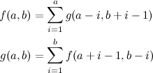
Then the main D.P. relation would look something like this:

Let’s see how it works; let’s consider the \(f\) relation that describes the “up” movements —the reasoning for \(g\) is very similar. We have to select one number from the \(A\) group. We have \(a\) different choices for this next movement, and this is represented by \(f(a, b)\). If we choose the smallest number in that group, then we leave two groups: a new \(A\) with \(a'=a-1\) elements and \(B\) remains the same. If we choose instead the second smallest number, then the groups change in size as follows: \(a'=a-2\) and \(b'=b+1\) (because by choosing the second smallest number, the very smallest number moves into the \(B\) group). The same thing applies for the third smallest number, the fourth, and so on, and that’s what the summations represent.

Going back to our example \(N=5, m=3\), we know we have two options for the second number of the sequence: we can pick 1 or 2. If we picked 1, the new situation would be:

\(A=(2, 4, 5) \;;\; B=() \;;\; a=3 \;;\; b=0 \;;\; n=1\)

If we picked 2 instead, it would be:

\(A=(4, 5) \;;\; B=(1) \;;\; a=2 \;;\; b=1 \;;\; n=2\)

All of this information is for illustration purposes, but you can notice that the actual contents of \(A\) and \(B\), as well as the last number picked \(n\) are irrelevant. The only thing that matters in our algorithm is the values \(a\) and \(b\) and whether the next movement has to be “up” or “down”.

Notice also that this process is guaranteed to end at some point because the total number of elements used as arguments for \(f\) and \(g\) are being decreased by one at each step. This leaves us with an algorithm that can compute all possible answers in \(O(N^3)\). This is a pre–calculation that happens only once in the program, and then each test case can be answered in \(O(1)\). If \(m > 1\) then the answer would be \(g(N-m, m -1)\). The small adjustment for the case \(m=1\) is left as an exercise for the reader :).

Wednesday, 12 September 2012

Tiles

Problem Name: Tiles
LightOJ ID: 1244
Keywords: recursion, matrix exponentiation

This is a problem involving an interesting recurrence that combines different inter–dependent relations. Moreover, given the large range of the input, it can be tackled with matrix exponentiation instead of classic dynamic programming.

You have a rectangular board of size \(2 \times N\) that is to be filled with tiles of six different types. 2 tiles are formed by two squares (each of size \(1 \times 1\)) and have the shape of a bar. The remaining 4 tiles have three squares, representing the four different rotations of a L–shaped tile. The tiles have to be placed in the board as–is (without rotating or flipping them).

We’ll identify the six tiles by the characters \(A, B, \dots, F\). This is how they look, using a single lowercase character to represent each square:

a      c   dd   e  ff
a  bb  cc  d   ee   f

The question is, in how many different ways can the board be filled using the six tiles?

It shouldn’t take long to see that it would be convenient to start by defining the following function:

\(f(n)\)
Number of ways to completely fill a board of size \(2 \times n\).

However, there is not a straightforward solution from just this relation —at least not one that I can see. Something that helps here is looking at a couple of additional “states” that can be analysed and used to build our final answer.

Consider the following auxiliary functions:

\(g(n)\)
Number of ways to fill a board of size \(2 \times (n-1)\), leaving a single square in the top row of the \(n\)th column.

and finally,

\(h(n)\)
Number of ways to fill a board of size \(2 \times (n-1)\), leaving a single square in the bottom row of the \(n\)th column.

Think for example of what happens when you have completely filled a section of the board of size \(2 \times k\), going from left to right, and you append a \(C\) tile. Then you have filled an area of \(2 \times (k+1)\), but you have an additional single square at the bottom of column \(k+2\). Those are the situations where \(g\) and \(h\) will prove useful.

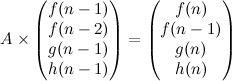
Also, having these three relations make it possible to now formulate a definition of \(f(n)\):

These expressions come directly from thinking about the different ways to place the six tiles inside the board. Let’s take \(f(n)\) for example. By definition, \(f\) concerns itself only with filling the first \(n\) columns entirely, so it shouldn’t include cases where the tile \(C\) and \(D\) are placed last. It only considers the cases where the last tile is either: \(A\), represented by the term \(f(n-1)\); or \(B\), which leads to \(f(n-2)\) (using two \(B\) tiles one on top of the other); or \(E\) and \(F\), which lead to \(g(n-1)\) and \(h(n-1)\) respectively.

The definitions of \(g(n)\) and \(h(n)\) come from a similar reasoning. Try to deduce them by yourself thinking about the different ways in which you can leave one single square in the last column. The beauty of this is that now all the terms show recurrence and lend themselves to a matrix exponentiation strategy quite nicely.

Let’s outline two of the three matrices, leaving the matrix with the coefficients for last:

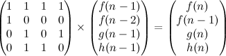
Now here’s the crucial step for our implementation. Given our previous definitions of \(f\), \(g\) and \(h\), we fill the matrix \(A\):

With this now we can write the implementation, and obtain the answer in \(O(k^3 log N)\), with \(k=4\).

Thursday, 6 September 2012

Aladdin and the Magical Sticks

Problem Name: Aladdin and the Magical Sticks
LightOJ ID: 1342
Keywords: math, probability, expected value, memoization, harmonic number

I’ve always had a keen interest in problems related to numbers, counting, probability and so on. It is only recently, however, that I’ve started to grow aware of the reasons why this might be so. Let’s take this problem as an example. After I read its description for the first time, I knew I would not rest until I found a satisfactory solution, and going into it I recognised that right then I still had some gaps in my knowledge, but still, it was thrilling to know that I was about to tackle something that would lead me to learn new things. It is a little hard to put into words, but there’s just something deeply enjoyable when you encounter a problem that you know you can’t yet solve, but your intuition tells you that you’re close; in other words, even if it’s a little beyond your current knowledge or skill, it’s within your reach. This is something that I’ve personally experienced with many math–related problems, and that’s probably the main reason why I find them fascinating.

Anyway, back to the subject at hand, this problem tells us the story of Aladdin, who is presented with a group of sticks, each one with a certain weight. He is asked to pick up the sticks, one by one, and every time he picks a stick, it is returned to the group and he has to continue picking sticks until all of them have been chosen. There’s a couple of extra details of importance: initially, the probability of picking any one stick is the same for all sticks, but, there’s also two types of sticks. One type is easily recognisable by Aladdin, so every time he picks a stick of this type, he doesn’t pick that same stick again. The other type of stick is normal and there is no way to recognise it, so sticks of this type could be picked many times. The question is: what is the expected weight of all the sticks Aladdin has to pick until all sticks have been chosen?

You may have noticed that this problem has a similar “flavour” to the Dangerous Maze problems —and they are, after all, from the same problem setter :). We could even rewrite the problem statement and use doors instead of sticks, and distances instead of weights, and the problems would look pretty similar. However, there is one crucial difference; in this problem you don’t “get out” until you have picked all sticks (or doors).

This difference turns this into an entirely different kind of problem. To give you some idea about the nature of the problems I’m talking about, think about how to calculate the expected number of throws of a single die until it shows a certain number, and how it differs from calculating the expected number of times you have to throw a die until you have seen all of its sides. Another way to look at it is to think about sticker albums or collectible card games. Let’s say that you can buy one card at a time, which comes completely at random (all cards with equal probability). How many cards do you need to buy until you complete your collection?

Not surprisingly, this is a classic conundrum known as the Coupon collector’s problem, and the math behind it is actually fairly accessible once you’re familiar with the basics of probability and expected value. Quoting from Wikipedia:

The key to solving the problem is understanding that it takes very little time to collect the first few coupons. On the other hand, it takes a long time to collect the last few coupons.

Let’s go back to the example with dice. Let’s say you want to know the expected amount of tosses until you have seen all sides from a standard die. You can split this problem into six sub–problems: how many tosses until you see the first “new” (previously unseen) side? How many tosses after that until you see the second “new” side? And so on until the sixth and final “new” side.

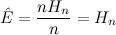
It’s easy to see that the first sides come up pretty quickly —you are guaranteed to see a new side on your first toss, and it’s very likely that you’ll see a new side on your second toss because the chance of repeating your previous toss is only \(1/6\). It’s the last unseen sides that take longer to come up. This leads to a very elegant formula for the expected value in the coupon collector’s problem. Using the terminology of this problem, if all sticks were of the second type (the type that is unrecognisable), then the expected amount of times that Aladdin would have to choose a stick until all of them were picked would be:

Where \(H_n\) is the \(n\)th harmonic number. At this point, I’d like to say that it’s very possible that you have now enough elements at your disposal to solve this problem. If you haven’t done so already, I suggest you take at least a couple of minutes right now to think about the mathematics of it, and try to formulate a solution —even a preliminary one. Nothing can replace that type of mental exercise.

Okay, now here’s what I found to be the final piece of the puzzle to arrive to my solution; it’s something I call “complementary” or “background–foreground” thinking (there’s probably a better name for it, but this is how I think of it). Edit: After re–reading some passages of one my favourite books ever —GEB— I can see that this concept is usually referred to as “Figure and Ground”. I’ll try to remember this…

Let me give you an example. Maybe you have confronted the Birthday paradox before, where you want to calculate the exact probability that any two people in a group of \(n\) people have the same birthday. You can approach this in two different ways, and one of them is going to be vastly easier than the other. You can try to go “straight” to the solution (what you see in the foreground) and consider every pair of people and the probability that they do have the same birthday. Obtaining the answer through this process is very complicated because of the relations formed between the pairs and the fact that you want to know the probability of any pair having the same birthday. The other approach is looking at the background or complement, and think of the probability that the \(n\) people have all different birthdays (let’s call it \(\bar{p}\)), and then your answer comes from the complement \(1 - \bar{p}(n)\). Much easier to calculate.

I hope the crux of the matter is clear. Sometimes if you can’t solve a problem looking at the foreground, it might be useful to look at the background and try to solve it from there. This is what I applied here. The idea is to initially consider all sticks as if they were of the second type; this gives us an initial expected weight \(W_i\). After that, subtract from \(W_i\) a weight from the sticks of type 1, proportionate to the “excess” in our calculation.

Why an “excess”? Well, it should be easy to see that if some of the sticks are of type 1, then our first estimation \(W_i\) is larger than the right answer, because no matter how we look at it, all sticks of type 1 are picked only once, no more. Let’s call \(\hat{E}\) the expected amount of times that one particular stick would be picked, if all sticks were of type 2. Then we have:

However, for sticks of type 1, this expected value is exceeded by the following amount (\(E_x\)):

Alright, now we can formulate the following algorithm:

  • Let \(A_T\) be the average weight of all the sticks.
  • Let \(E\) be the expected number of sticks that have to be picked (if all were of type 2). This comes directly from the coupon collector’s problem as \(E=n \cdot H_n\).
  • \(W_i = A_T \cdot E\)
  • If there is one or more sticks of type 1:
    • Let \(N_1\) be the number of sticks of type 1 and \(A_1\) the average weight of the sticks of type 1.
    • \(W_f = W_i - N_1(H_n - 1) \cdot A_1\)
  • Else, \(W_f = W_i\)

Our answer is \(W_f\).

Thursday, 30 August 2012

Turn the Lights Off

Problem Name: Turn the Lights Off
UVa ID: 10309
Keywords: brute force

I find this problem interesting for a number of reasons, but the first that comes to mind is that it involves a game with simple rules which anyone can pick up quickly, but its mathematical analysis is not trivial at all —and games of this kind are just fantastic, aren’t they?

Let’s start by mentioning that the solution I implemented can be classified as “brute force”, but if you think that it’s a naive brute–force (\(2^{100}\)), then we’re not on the same page, yet.

Actually, the first thing I did when I first read this problem was thinking about all the types of “blind” strategies and possible pruning that could be performed while looking for the solution through a breadth–first search. The results were not very encouraging. As you may have noticed, the space of possibilities is insanely large (\(2^{100}\)) and a BFS could end up using equally lunatic amounts of memory. The problem boils down to the simple fact that representing a “state” for this problem is not cheap: a boolean matrix of size \(10 \times 10\) is simply too much for any simple–minded approach.

Now, fortunately for us, some pretty smart people have worked hard on analysing this game in the past, and we can read about their findings through the magic of the Web :). First of all, as far as I know, the original game that implemented these mechanics is called Lights Out and was developed by a company called Tiger Toys in 1995, in case you want to do some research by yourself. If you do, one of the first website you’ll probably come across is this: Jaap’s Puzzle Page, which has a lot of information about it. There’s a related page dedicated exclusively to the mathematics behind Lights Out, which are fascinating to read about, but I won’t mention here mainly because my solution didn’t involve any sophisticated math analysis.

What I do want to mention though, is that there exists an heuristic that can be used to solve these puzzles, which can be summarised like this: press some buttons (i.e. switch some lights) from the top row, then “chase the lights” from the second row to the bottom. What this means is, starting with the second row, press a button only if the light to the north of the current position is on. Go on like this row–by–row until you reach the bottom. If in the end you haven’t cleared the grid, then go to the beginning, pressing some buttons from the top row, and repeating the process until you have solved it. Interesting, right?

But it gets better. In a paper —referenced in Jaap’s page— called “Turning Lights Out with Linear Algebra” we can find the following good news:

Lights Out can be generalized to an \(n \times n\) array of lights. (…) Of course if the dimension of the null space is zero, every configuration is winnable and the solution is unique (if no buttons are pressed more than once).

And then there’s a table where we find that the dimension of the null space for games of size \(10 \times 10\) is zero. In other words, for this problem, every configuration has a solution, and if we find it by “pressing a switch” no more than once, then it’s guaranteed to be the best solution.

Now we’re ready to formulate our solution: if we try pressing every combination of lights from the top row and then “chase the lights” downwards, we have to check only \(2^{10}\) alternatives, which are guaranteed to be enough to find our answer. I was truly amazed by how nicely this idea translates into elegant code, and it has a complexity of \(O(2^n n^2)\) (where \(n=10\) for this problem).

By the way, if you have some time to spare, maybe you’d like to give the heuristic explained here a try, on a game of “Lights Out” where the size of the grid increases at each level: here’s the game of Tacoyaki+. Have fun :).


References

Tuesday, 14 August 2012

Olympic Swimming

Problem Name: Olympic Swimming
UVa ID: 11546
LightOJ ID: 1423
Keywords: sweep line, hashing

The London 2012 Olympics closing ceremonies took place just a couple of days ago, and it has given me a nice excuse to work on a problem that somehow involves an Olympic event :). Actually, I had this problem near the front of my queue of “to do” problems and it coincidentally emerged during these days of “Olympics fever”. The real reason I find it noteworthy, however, is that it also gives me the opportunity to talk about a couple of interesting concepts that I have not talked about in previous posts.

The problem can be summarised as follows: imagine a swimming pool with length L metres (\(L \in \mathbb{Z}\)). This pool has K lanes, and marks at every metre, so you can imagine it as the sum of \(L\) sections, each one 1 metre long and with \(K\) lanes. The pool has a number of hurdles or obstacles (it doesn’t make much sense in real swimming events, but never mind that), such that each hurdle is placed on a particular lane, between two consecutive marks.

The question is, if you can divide the pool only at a mark, what is longest possible segment of the pool in which all the lanes have the same number of hurdles (not necessarily at the same locations)?

Let’s start by looking at an example to help us analyse this problem. Consider a pool of length 10 and with three lanes. The lanes will have 3, 4 and 2 hurdles, as depicted in the following figure:

Try to find two marks \((i, j)\) such that all lanes have the same amount of hurdles in that segment of the pool and \(j - i\) is maximised. After some trial and error, it should become clear that the longest segment is \((5, 9)\), with a length of 4 and one hurdle per lane.

Now we can discuss the first interesting concept that this problem leads us into, which is the sweep line algorithm. The idea behind this is simple (although the specific details for certain problems might not be simple at all): you have a geometric plane and a set of points that relate to your model of a problem; you use an imaginary line that is moved over the plane, and every time it hits one or more points, some type of calculation is performed. In this way you’re computing a certain value gradually with an algorithm that has, at first, a complexity of \(O(n)\) —not counting the operations you perform at each “collision”. This type of algorithm can be applied to many interesting geometry–related problems, like finding the closest pair of points in a set (see problem UVa 10245) or computing the outline of the union of a set of rectangles with a common baseline (see problem UVa 105).

We’ll apply the general principle to this problem, but first let us give it a little more thought and find out how a sweep–line strategy may be useful. One of the first things to notice is that if you start at the mark \(i=0\) and move forward all the way to \(i=L\), the number of hurdles at each lane can only increase or stay the same at each step, so maybe a prefix sum can help us get closer to the answer. Let’s start by defining the following:

\(P_{i}\)
A tuple with the prefix sums of hurdles at position \(i\). Each element in the tuple corresponds to one lane.

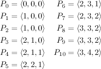
According to this definition, the values of \(P\) for our example are:

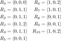
Do you notice anything particularly interesting in this list, keeping in mind that we know that our answer is in the segment \((5, 9)\)? You should see that the relative differences among the elements in \(P_5\) are the same as in \(P_9\). In fact, those two tuples form the pair that is the most distant while having the same relative differences internally. To see it more clearly, let’s bring a second definition that simplifies things for us:

\(R_i\)
A tuple where each element \(R_{i, j} = \text{max}(P_i) - P_{i, j}\)

Now we have enough elements to formulate our main algorithm. If we use a sweep–line, we could calculate \(R_i\) and \(R_{i+1}\) at each point \(i\) given in the input and every time we find an \(R\) tuple that we have seen before, we calculate the distance between the new mark and the old mark, and our final answer comes from choosing the overall maximum.

This brings us to the second concept that I want to talk about —hashing. You see, a sweep line by itself is just a very basic approach, but what’s important is the type of operations you do at each critical point you find in your sweep, which commonly requires keeping track of data (inserting, querying, deleting) very quickly. For this reason, a sweep line algorithm usually comes along with some kind of efficient data structure such as B-trees or hash maps.

In Java you could use a java.util.HashMap (implemented internally using a hashing algorithm) and in C++ you could use STL’s map (implemented internally as an ordered tree) or use you own hashing algorithm. Given the tight time limit constraints for this problem (at least in the UVa judge), it’s probably better to use your own hashing algorithm. For a good introduction to many good hashing algorithms (and hashing in general), you can read this excellent article: The Art of Hashing.

I’d recommend you choose a simple algorithm, one that doesn’t perform many computations per byte. Some good ones are the Bernstein hash, the Shift-Add-XOR hash and the FNV hash. I personally use the FNV algorithm, but in practise they tend to perform very similarly.

I will not post the code for a hash table here because if you are about to write your own hash map implementation for the first time, I think it would be better to do it from scratch and use it as an exercise to learn the concepts in depth (and also you end up with something written in your own style). However, I’ll give you the general idea of how all of this glues together.

First, you have to implement your hash table. There are many ways to do it but a fairly simple and effective method is keeping a number of “buckets” to place your data into, and for any piece of data you want to store, you find its corresponding bucket using your hashing algorithm. The right amount of buckets to use depends on the problem, your hashing algorithm and the size of your input, but I’ve seen that you quickly reach a point where using more buckets doesn’t have any significant impact in the efficiency of your program, so you don’t need to choose a very big number. For this problem, for example, I’ve used \(2^{15}\). Since you have to assume that in general there will be collisions in your hashing procedure, each bucket is, in reality, a linked list (or vector) of data. Don’t worry if you think that using linked lists will be slow. When you have a fairly decent hashing algorithm, the number of collisions should be minimised, and the resulting average complexity is really good, perhaps even an order of magnitude better than using other data structures like trees in your buckets because of the minimal overhead of using a linked list or vector.

With your hash table in place, you apply the sweep line strategy. To put it all together, the algorithm for this problem could look something like this:

  1. Read the data that describes the pool, and sort the hurdles, first by their mark \(p_i\), and then by their lane.
  2. Let \(A=0\), where \(A\) represents our final answer.
  3. Let \(R\) be the tuple \(\langle0, 0, 0\rangle\). Add \(R\) to your hash table, associated with the value 0 (the mark that corresponds to the tuple \(R\)).
  4. Sweep line. For each hurdle in your data:
    1. Let \(m\) be the mark of the current hurdle. The tuple \(R_m\) is the same \(R\) we had previously, so calculate the difference \(d = m - \text{HT}(R)\) where \(\text{HT}(R)\) is the value associated to \(R\) in the hash table. Let \(A = \text{max}(A, d)\).
    2. Take from your input all other hurdles that are also at \(m\), and with that calculate \(R_{m+1}\).
    3. Add the new \(R\) to the hash table associated with the mark \(m+1\). If \(R\) was already in the table, calculate \(d = m + 1 - \text{HT}(R)\) and \(A = \text{max}(A, d)\).
  5. In the end, the current \(R\) should be the value of \(R_L\), so calculate \(A = \text{max}(A, L - \text{HT}(R))\).

The final value of \(A\) should be our answer. Our resulting algorithm starts by sorting the input —with a complexity of \(O(n K \log{n K})\)— then does a sweep line (\(O(n)\)) with a hashing algorithm at each critical point (\(O(K)\)), which gives us an overall complexity of \(O(n K \log{n K})\).

Friday, 3 August 2012

Goldbach and Euler

Problem Name: Goldbach and Euler
UVa ID: 10311
Keywords: number theory, primes, sieve

When you come across a problem titled after two well-known, brilliant mathematicians, you know it’s going to be good :).

What the problem is asking for can be expressed as follows: given an integer n (which can go as high as 108), find —if possible— two prime numbers p1 and p2 such that:

  • \(p_1 + p_2 = n\)
  • \(p_2 > p_1\)
  • \(p_2 - p_1\) is minimised

It is clear that for this problem it is necessary to find out which numbers are primes in the range \((0 : 10^8)\). Let’s focus on that first.

As you probably know, one good way to find prime numbers computationally is using the classic Sieve of Eratosthenes (or a similar but possibly faster alternative, such as the Sieve of Atkin). No matter what kind of “sieve” you use, you have to implement it in a way that allows you to store information about 108 numbers, which is not a trivial job.

Let us generalise the problem and say that you want to find all prime numbers up to an integer N. If you write a regular implementation using a boolean (bool in C++ or similar) data type for each integer in the range [1:N] then you would end up using N bytes of memory, which for this problem would mean about 95MB —just “a tad” heavy.

Fortunately, there are ways to reduce the memory requirements with relatively few changes that are easy to code. The main idea is that a boolean value can be stored in a single bit, so you can store 8 boolean values in a single byte. In addition, consider that most prime numbers are odd; in fact, there is only one even prime number which is 2. With this in mind, you can further cut your memory requirements in half by simply not storing information for even numbers (you have to handle the case of 2 separately, of course).

So, with these adjustments, we can now implement a prime-finding sieve that requires only \(N \div (8 * 2)\) bytes. If we store this information in 4-byte integers, then we require only \(N \div 64\) integers. The following is a C++ implementation of this type of sieve, using the standard Eratosthenes algorithm, which has served me well for some time:

const int MAX = 100000000;  // 10^8
const int LMT =     10000;  // sqrt(MAX)

// array of data; each bit tells if a certain number is composite or not
int _c[(MAX>>6)+1];

// we use a STL vector to store the primes
vector<int> primes;

// possibly the most important piece for a bitwise sieve
// these are the macros that check and set a bit
#define IsComp(n)  (_c[n>>6]&(1<<((n>>1)&31)))
#define SetComp(n) _c[n>>6]|=(1<<((n>>1)&31))

void prime_sieve() {
    for (int i = 3; i <= LMT; i += 2)
        if (!IsComp(i))
            for (int j = i*i; j <= MAX; j += i+i)
                SetComp(j);

    primes.push_back(2);
    for (int i=3; i <= MAX; i += 2)
        if (!IsComp(i))
            primes.push_back(i);
}

bool is_prime(int n) {
    if (n < 2 || n % 2 == 0) return false;
    return ! IsComp(n);
}

As you can see, this implementation reserves about \(10^8 \div 64\) integers for the main array, which represents about 6MB of memory, a good deal better than the original 95MB. However, it also uses memory to store the actual prime numbers in a vector. Since there are about 5.8 million primes under 108, then this would require an extra \(4 \times 5.8 \times 10^6\) bytes (about 22MB).

Having solved the problem of calculating and storing the primes, now let’s move on to the problem of finding \(p_1\) and \(p_2\). The first idea that comes to mind is something like simply trying to find \(p_1\) starting with \(n \div 2\) and going downwards, checking that \(p_1\) and \(p_2 = n-p_1\) are primes.

However, it’s easy to see that this simple idea would take too long in practise. There’s one thing that we could do that would improve significantly the complexity of the algorithm, which is not iterating through all integers, not even through odd integers only, but only over the prime numbers. Since we already have a vector full of primes below 108, we can binary search the location of \(n \div 2\) and go down from it. That would make for a worse case of \(5.8 \times 10^6\) iterations instead of \(10^8 \div 2\).

We have improved things but, can we do even better? The discussion found in the problem statement about Goldbach’s conjecture and Euler’s ideas on the subject is very interesting on itself, but it also points to something that could be useful: an even number can always be expressed as the sum of two primes (well, it’s a conjecture, but it has been tested for a range of numbers much larger than \((0 : 10^8)\), so we can assume it’s true for our purposes). This means that we can be reasonably confident that the process of finding \(p_1\) will succeed for most even numbers, hopefully quickly enough that it doesn’t have to check millions of primes. Note that I said most even numbers; this is because we need two distinct primes \(p_1\) and \(p_2\), remember? For example, 6 can be expressed as the sum of two primes (3 + 3) but not as the sum of two distinct primes.

Okay, we have concluded that for even numbers our algorithm may not be so bad, but what about odd numbers? Well, it turns out that for odd numbers the algorithm can be \(O(1)\)! If \(n\) is odd, then one of the two primes \(p_1\) and \(p_2\) has to be even, while the other has to be odd (if you don’t see this clearly, think about how even numbers are integers of the form \(2k\) and odd numbers are integers of the form \(2k + 1\)). Do you see where this is going? If one of the primes has to be even, then that prime would have to be 2 (there are no other even primes). So, if \(n\) is odd we simply check if \(n-2\) is prime, and if it is, then we know that \(p_1=2\) and \(p_2=n-2\), otherwise there is no solution.

We have covered all possible cases now, and after testing it, it produces an answer reasonably fast. Prime numbers are lovely :).