Rip Van Winkle's Code

Problem Name: Rip Van Winkle’s Code
UVa ID: 12436
LightOJ ID: 1411
Keywords: segment tree, lazy propagation

Today we’ll take a look at a problem from this year’s ACM ICPC World Finals Warmup contest, and which can be solved with the help of segment trees. It will give us an opportunity to contemplate some more of the nice subtleties that often come into play in this type of problem.

We’re asked to consider an array of 64–bit integers. The size of this array is fixed at 250,001 positions (index 0 is left unused, so we have to focus only on positions 1–250,000) and it is initially filled with zeroes. Three types of operations can modify this array:

• Operation A takes two integers, let’s call them \(i\) and \(j\), and adds 1 to position \(i\) of the array, 2 to position \(i+1\), 3 to \(i+2\) and so on. In other words, it increases the values in the range \([i:j]\) of the array according to the sequence \(1, 2, 3, \ldots, (j-i+1)\) from left to right.
• Operation B is similar to A, but it applies the additions in a right–to–left fashion (it adds 1 to position \(j\), 2 to position \(j-1\) and so on).
• Operation C is simpler. It also takes two integers that describe a range, but it receives an extra argument; an integer \(x\). All positions in the range \([i:j]\) of the array are then set to \(x\).

Finally, we have a fourth operation S which doesn’t alter the array, it must simply report the sum of all positions in a given range \([i:j]\) of the array.

Let’s quickly illustrate these operations with an example. We’ll consider the arbitrary range \([120:127]\) of the array. At first, this range looks like this:

Now, let’s say that we receive the following commands to execute in order:

• A 123 126
• A 122 124
• B 120 127
• C 125 127 3

Then the changes inside the data array would look as follows:

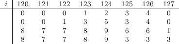
Okay, now that we’re a bit more familiar with the problem, let’s give it some thought. As I mentioned in the beginning, we’ll base our approach on the powerful segment tree data structure. With this in mind, it would seem that implementing operations C and S could be fairly straightforward. However, operations A and B are somewhat tricky. They modify a range of values, but each position in that range is modified differently. We should, however, try to implement those commands in a way that involves just one update on the tree (with complexity \(O(\log{N})\)), otherwise our code wouldn’t be too efficient.

Let’s start by visualising our segment tree for the small range we chose in our example. We’ll start with the basics, just storing in each node of the tree the total sum of the corresponding range. We’ll extend this tree gradually as we see fit.

This tree represents the range \([120:127]\) of a fresh array, so it’s filled with zeroes. The first row in each node contains its index and range, while the second row contains the sum of all positions in the corresponding segment in the array. Notice that the nodes of this tree have been indexed using the numbers \(1, 2, \ldots, 15\), but in reality these nodes would receive different indices —node 1 would be for the real root of the tree, which covers the range \([1:250,000]\), node 2 would be its left node, and so on. Numbers 1 to 15 are used here just to simplify things a bit in the following examples, but keep in mind that they would not be the real indices in the segment tree for the whole array.

Alright, let’s consider our first query: A 123 126. How would the tree be affected by this command? We could produce something that looks like this at first:

By looking at this tree, a few things are brought to our attention. One is that the value of each affected node is increased according to a sequence of consecutive integers, but the sequence is of course different for each node. For example, node 6 was increased by 5, which is the result of \(2+3\). For that node, the sequence applied to increase the values in the range \([124:125]\) started with 2, and its length is 2 of course. Another important thing that this graph seems to “shout” at us, is that we must devise a strategy for the propagation of this update. The situation is pretty evident in nodes 12 and 13. How can we tag these nodes so they are properly updated down the road?

But let’s pause for a second and think on the situation of sequences of consecutive integers that start with an arbitrary number. We’ll generalise and consider a node that represents a segment of length \(k\). The contents of the node (the sum of all values in its range) will be denoted \(S\). When we receive an A operation that affects this node, we have to change its contents according to a sum of the form:

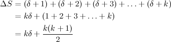
Where \(\delta\) represents the distance of each element in the base sequence \(1, 2, 3, \ldots, k\) to the corresponding element in the actual sequence applied to the node, which could start with any positive integer. To illustrate this, we can see in the graph above that, for node 11, \(k=1, \delta=0\); for node 6, \(k=2, \delta=1\); and for node 14, \(k=1, \delta=3\).

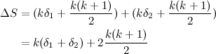
This method of representing the A operation has also the benefit of working out nicely when we accumulate the results from more than one command of this type for the same node. The value of \(k\) remains the same in each node, so the only thing that could change is \(\delta\). Let’s say that a certain node receives two A operations, one after the other, with two values \(\delta_1\) and \(\delta_2\). This would result in the following:

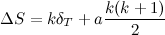
In general, if a node receives \(a\) operations of type A, with a total \(\delta_T\) —the result of adding \(\delta_1, \delta_2, \ldots, \delta_a\)— then all these changes can be represented by the expression:

And what about the B operation? Well, if you think about it for a minute, it should be easy to notice that it works very similarly to an A operation. The difference is that the \(\delta\) values are calculated differently (right to left) and that, in order to facilitate the calculation of \(\delta\) values for children nodes, it would be convenient to keep track of the number of B operations with a different variable (let’s call it \(b\)).

Putting all of this together, we can now extend each node of the segment tree with three additional values: \(a\) (the number of A operations to propagate), \(b\) (the number of B operations to propagate), and \(\delta\) (the sum of all \(\delta\) values from either A or B operations). Let’s see how our tree looks like now:

What is nice about this approach is that, given that every node is implicitly associated with a given range of the array, it is easy to determine the values of \(k\) and \(\delta\) in each node (and their children) for every A and B operation. And calculating the new \(S\) from \(a\), \(b\) and \(\delta\) is even easier.

Let’s quickly review how the tree changes with the rest of the operations we used in our original example. After the operation A 122 124 we would have:

And after B 120 127:

Note that, as I mentioned in the analysis of Ahoy, Pirates!, there are some things that happen behind the curtains while propagating updates down the tree. For example, when the second A operation is issued, the tree is traversed down to node number 12, and in the process node 6 and its children are visited, and that’s when node 13 is updated so its \(S\) value becomes 3, while \(a, b, \delta\) are cleared.

Now we have only one operation left to implement: C. We could try to implement it using the \(\delta\) field we have already defined, but that would represent some difficulties when several commands are stacked for future lazy propagation. Consider for example a C command followed by an A operation and vice–versa. To avoid these issues, and for commodity, we’ll simply create a couple of new fields: one boolean field \(c\) that represents whether a C operation is pending or not, and a field \(x\), which is simply the argument for the corresponding C operation.

Let’s see this new extended tree, and how it would change after the command C 125 127 3:

Once again, a few nodes have changed purely as a side–effect of traversing the tree (e.g. nodes 2, 4 and 5). It’s also worth mentioning that once a C operation is passed on to a child node for lazy propagation, the \(a\), \(b\) and \(\delta\) fields of the child are cleared, because the C operation overrides any previous commands. This can be seen, for example, in nodes 14 and 15. However, A and B do not override previous commands.

---

Okay, we have reached the end of this analysis. I’d like to end by commenting on something that I realised while working on this problem, which is that I’ve developed a special appreciation for algorithm problems related to segment trees, because they typically require a little bit of… I guess you could call it “inspiration”, to nail the right representation of the relevant data and to imagine how every operation should work and be propagated through the tree. Not only that, these problems also demand a lot of attention to detail in the implementation, because with so many subtle things to keep track of, it’s easy to make a mistake somewhere.

How nice it is that we all have the opportunity to sharpen our skills by working on fun problems like this one :).

Ahoy, Pirates!

Problem Name: Ahoy, Pirates!
UVa ID: 11402
Keywords: segment tree, lazy propagation

Working on algorithm problems has been one of my favourite hobbies for a while now, and I’m constantly inspired by the fact that, although there is a finite (and not too large) set of concepts that cover the landscape of all possible problems you can encounter, in practise it feels like there are no boundaries to the amount of things you can learn. In a very real sense, you can always keep learning new things, and the more you learn, the more you find new things that you want to learn next.

I still have many gaps in some basic areas, so I like diving into new things whenever I have the chance to do it. For example, it’s only recently that I have learned a little about a few data structures that were a mystery to me for a long time; segment trees, binary indexed trees, sparse tables, k-d trees… For this reason, I think the next few entries I’ll write for this blog will be for problems related to these data structures. I’ll start with the segment tree by having a crack at this problem —Ahoy, Pirates!— which I think is a very nice exercise for developing a deeper understanding of a ST and the subtleties of implementing update operations on it.

The Problem

Consider a large array of boolean values, represented as zeroes and ones. You have to implement four types of operations that can be performed over this array:

1. Set, or “turn on” a range of adjacent positions in the array (set them to 1).
2. Clear, or “turn off” a range (set to 0).
3. Flip a range (turn zeroes into ones and vice–versa).
4. Query the number of ones in a given range.

Very interesting problem, if you ask me. We’ll begin with a simple example, as usual. Let’s say we start with an array \(A\) of size 8, and with the following contents:

Querying, First Approach

Now, let’s say we receive a query that asks for the number of ones in a range \([i:j]\) with \(0 \leq i \leq j < N\), where \(N\) is the size of the array (8 in this example). One simple idea is to simply traverse the array with a loop from \(i\) to \(j\), counting the number of ones in the way.

That would be an acceptable solution if that were the only query to answer, or if the number of queries were very low. However, given that the array is big, and there’s a relatively large number of queries, a complexity of \(O(NQ)\) is too high for our needs.

What we’ll do instead is use a segment tree. This is a very nice data structure where a binary tree (typically a binary heap) is built on top of an array in order to store useful information from the underlying data in groups of increasing size. The leaves of the tree correspond to the individual positions inside the array, while internal nodes represent data that is the result of combining information from its children. The root corresponds to an interval that encloses the whole array.

Let’s try to visualise this with our example:

This graph depicts three things for each node in the tree: its interval (enclosed in a purple box), its index (in red) and its contents (in blue), which in this example corresponds to the number of ones in the corresponding interval. Note the convenient way in which the indices of all nodes are related to each other, as is common in heap–like data structures. In this case, the convention is that for a node \(i\), its two children have indices \(2i\) and \(2i + 1\). As you can see, although this data structure represents a tree, it can be stored in a plain array of size 16 (index zero is left unused).

Now, consider why building something like this is useful. If we receive a query that asks for the number of ones in the whole array, we don’t need to go any further than the root of the tree; in other words, an operation that would have taken us \(N\) steps with a common loop, takes us only a single step now. Similarly, if we’re asked about the range \([0:3]\), we just need to visit two nodes: the root and its left child.

Some queries may involve combining the answer from different paths. For example, if we have a query for the range \([2:6]\) then the following nodes of the tree would have to be visited: 1, 2, 5, 3, 6, 7 and 14. This might seem like a bad trade–off in this small example, but it is a huge gain in general. In fact, it’s easy to see that the complexity for an arbitrary query goes from \(O(N)\) to \(O(\log{N})\).

Updating the Tree

So far so good, but what would happen if we try to update the tree after it has been built? Let’s focus on just the Set operation for now.

For the reasons we have discussed before, we should avoid updating the underlying array and then re–building the whole tree; that would have an excessively high complexity. Instead, we can observe this: since every node is implicitly associated with an interval of the array, it’s easy to find out how many positions it covers, and that way we can easily determine the new contents of each affected node after a Set operation.

Back to our example. Let’s say that we receive a query that asks us to set the range \([1:7]\). This is how it could look like just after the relevant nodes have been updated:

The update process (as any operation performed on a ST) starts with the root. The tree is traversed downwards via recursive calls until a node that is completely contained in the relevant interval is found. Those nodes are then updated first (the nodes with blue background). The changes then propagate upwards, as the recursion stops and the stack is popped back until we’re back at the root again (these changes happen in the nodes with gray background).

In this example we can see how, for example, the path from the root to node 9 seems fine and needs no adjustments. Same thing with the sub-tree at node 5, but only by chance, because the contents of that node didn’t change (the range \([2:3]\) of the array already had two ones). However, notice the resulting situation for node 3. At this point, if we received a query asking for the number of ones in an interval that completely contained the range \([4:7]\), we’d have no trouble to find the answer; the information of the root and node 3 is correct. However, the sub–tree at node 3 is inconsistent. If, for instance, we received a query for the interval \([4:5]\), we’d reach node 6 and find the old value of 1 there, which is not correct.

Lazy Propagation

It has been said —by notoriously bright people— that laziness is one of the three great virtues of programmers. As it turns out, laziness is also a desirable property for algorithms. When we update the tree, we don’t want to always propagate the changes down to the leaves (which would be even worse than just updating the original array of integers in a loop). However, we don’t want to leave the tree in an inconsistent state either.

The solution is to extend the tree with an extra field that indicates whether the relevant sub–tree needs to be updated or not. This way, nodes in the tree are properly updated as needed by future queries, and not a moment before; hence the lazy name.

We will extend our tree, then. Since we have three types of operations that change the tree, we’ll store a flag that stores one of four possible values: S for a set operation, C for a clear operation, F for a flip operation, and N for nothing, meaning that the current node is up–to–date —unless one of its ancestors is not N, but that would be handled in due time. This is how our example would look like after the update, with the extended information (there’s a new state field in green):

This tree, unlike the previous one, has now enough information to maintain a consistent state at all times. Note that now nodes 10, 11, 6 and 7 are marked with S, meaning that the next time they are visited, a Set operation will be propagated (lazily) from them. We could have left nodes 10 and 11 untouched because, as has been mentioned, node 5 didn’t change, but we’ll leave them marked just to illustrate the basic process without special checks.

At this point, let’s say that we received a query asking for the number of ones in the range \([4:5]\). This time node 6 is visited, but since it’s marked S, then first we’d have to propagate the Set operation, which means updating the contents of node 6 itself, and then marking its children so the lazy propagation continues with them if necessary. This continuous propagation of previously marked nodes ensures that the information of the tree is always correct, without updating more nodes than necessary. A very powerful technique.

In order to illustrate the operations we haven’t considered yet, let’s say that we also receive a query to Clear range \([7:7]\), and a query to Flip range \([0:3]\). This is how the tree would look like after all these operations:

Okay, to summarise, this is what we’ve imagined so far in our example:

• Building the tree.
• A Query for range \([0:7]\). The result is 4 and is obtained just by looking at the root.
• Queries for ranges \([0:3]\) and \([2:6]\). They need to visit more nodes of the tree, but the result is still obtained in \(O(\log{N})\).
• A Set operation for the range \([1:7]\). It updates directly nodes 9, 5 and 3, and their ancestors, and marks their children so they are lazily updated in the future.
• A Query for range \([4:5]\). This updates node 6 (because it was marked S), and marks its children for future propagation.
• A Clear operation for range \([7:7]\).
• A Flip operation for range \([0:3]\).

The “array” (which lives now inside our ST) now has a total of four ones, yet this is not clear from looking at the leaves alone. You need to analyse the internal nodes to understand how is it that this array has been modified, and what updates have not been propagated yet.

But wait a minute, did you notice how node 14 has a one now, and its state is N? When did that happen? Then answer is, it happened in the middle of the Clear for \([7:7]\). The sequence of events was like this:

1. A Clear for \([7:7]\) was requested.
2. The tree is traversed from the root, and it goes recursively down to nodes 3 and 7. At this point it finds that node 7 is marked S.
3. It propagates this change, which means changing the contents of node 7 to 2, and marking its children (nodes 14 and 15) with S.
4. Immediately after that, it continues with its original request, but to handle it, it has to visit 7’s children first, so it goes down to nodes 14 and 15.
5. This is when the changes happen. I had not mentioned this before, but the way the tree is traversed, it needs to keep visiting nodes, until either a node is completely inside the relevant interval (like node 15 here), or it’s completely outside the interval (like node 14 here). So, node 14 is visited, and since it’s marked S, it changes its value to 1, resets its state to N and it stops traversing this branch.
6. Node 15 is updated according to the Clear request, and stops there as well.
7. All these changes propagate back upwards, resulting in the tree you see in the last figure.

I hope this overview has helped you in case you haven’t worked with segment trees before.

I want to end this by mentioning a curious detail that applies to this specific problem as a result of the operations it involves. Consider the situation of nodes 5, 10 and 11 in the last figure. Node 5 is marked F and its children are marked S. Now consider what would need to happen if, for example, you receive a query for range \([2:3]\). In other words, think about what happens if a node \(u\) with state \(s(u)\) is visited, and one of \(u\)’s children is node \(v\) with state \(s(v)\). How should state \(s(u)\) be propagated down to \(s(v)\)?

There’s a few alternatives:

• If \(s(u)\) is N, then nothing needs to happen.
• If \(s(u)\) is S or C, those operations are overriding, meaning that the state of \(v\) must be set to \(s(u)\) regardless of the previous contents of \(s(v)\).
• However, if \(s(u)\) is F, then the previous contents of \(s(v)\) are important, and they need to change accordingly:
  • If \(s(v)\) was N, it becomes F.
  • C becomes S.
  • S becomes C.
  • F becomes N.

Kinda cool, isn’t it?

Sample Code

I usually don’t include source code in my posts because I prefer describing the general algorithms, but in this case I’ll attach the basics of my segment tree code for this problem, because I know that finding reference code for this data structure on the web can be a little difficult.

This code con be simplified much further by combining similar code from different methods, but this way you can see how every individual operation is implemented separately, and it also makes it easy to identify the common patterns of manipulating the segment tree.

#define MAXN 1024000
#define MAXH 21  // 1 + ceil(log2(MAXN))

// Flags to identify states. 0 is for "Nothing".
#define UP_SET 1
#define UP_CLR 2
#define UP_FLP 3

struct SegTree {
    vector<int> A;  // original array of integers
    vector<int> T;  // segment tree
    vector<int> U;  // segment tree for lazy propagation (the states)

    int n;  // size of the array

    SegTree(int N=0) : n(N) {
        A.resize(MAXN);
        T.resize(1 << MAXH);
        U.resize(1 << MAXH);
    }

    void init() { tree_init(1, 0, n-1); }
    void tree_init(int x, int a, int b) {
        U[x] = 0;
        if (a == b) { T[x] = A[a]; return; }
        int lt = 2*x, rt = lt + 1, md = (a+b)/2;
        tree_init(lt, a, md);
        tree_init(rt, md + 1, b);
        T[x] = T[lt] + T[rt];
    }

    void set(int i, int j) { tree_set(i, j, 1, 0, n - 1); }
    void tree_set(int i, int j, int x, int a, int b) {
        propagate(x, a, b);
        if (j < a || i > b) return;
        if (a == b) { T[x] = 1; return; }
        int lt = 2*x, rt = lt + 1, md = (a+b)/2;
        if (a >= i && b <= j) {
            T[x] = b - a + 1;
            U[lt] = U[rt] = UP_SET;
            return;
        }
        tree_set(i, j, lt, a, md);
        tree_set(i, j, rt, md + 1, b);
        T[x] = T[lt] + T[rt];
    }

    void clear(int i, int j) { tree_clear(i, j, 1, 0, n - 1); }
    void tree_clear(int i, int j, int x, int a, int b) {
        propagate(x, a, b);
        if (j < a || i > b) return;
        if (a == b) { T[x] = 0; U[x] = 0; return; }
        int lt = 2*x, rt = lt + 1, md = (a+b)/2;
        if (a >= i && b <= j) {
            T[x] = 0;
            U[lt] = U[rt] = UP_CLR;
            return;
        }
        tree_clear(i, j, lt, a, md);
        tree_clear(i, j, rt, md + 1, b);
        T[x] = T[lt] + T[rt];
    }

    void flip(int i, int j) { tree_flip(i, j, 1, 0, n - 1); }
    void tree_flip(int i, int j, int x, int a, int b) {
        propagate(x, a, b);
        if (j < a || i > b) return;
        if (a == b) {
            T[x] = T[x] == 1 ? 0 : 1;
            return;
        }
        int lt = 2*x, rt = lt + 1, md = (a+b)/2;
        if (a >= i && b <= j) {
            T[x] = (b - a + 1) - T[x];
            U[lt] = apply_flip(U[lt]);
            U[rt] = apply_flip(U[rt]);
            return;
        }
        tree_flip(i, j, lt, a, md);
        tree_flip(i, j, rt, md + 1, b);
        T[x] = T[lt] + T[rt];
    }

    int query(int i, int j) { return tree_query(i, j, 1, 0, n-1); }
    int tree_query(int i, int j, int x, int a, int b) {
        if (j < a || i > b) return -1;
        propagate(x, a, b);
        if (a >= i && b <= j) return T[x];
        int lt = 2*x, rt = lt + 1, md = (a+b)/2;
        int q1 = tree_query(i, j, lt, a, md);
        int q2 = tree_query(i, j, rt, md + 1, b);
        if (q1 < 0) return q2;
        if (q2 < 0) return q1;
        return q1 + q2;
    }

    int apply_flip(int v) {
        if (v == UP_SET) return UP_CLR;
        if (v == UP_CLR) return UP_SET;
        if (v == UP_FLP) return 0;
        return UP_FLP;
    }
    void propagate(int x, int a, int b) {
        if (U[x] == 0) return;
        if (U[x] == UP_SET)
            T[x] = b - a + 1;
        else if (U[x] == UP_CLR)
            T[x] = 0;
        else if (U[x] == UP_FLP)
            T[x] = (b - a + 1) - T[x];

        if (a != b) {
            int lt = 2*x, rt = lt + 1;
            if (U[x] == UP_SET || U[x] == UP_CLR)
                U[lt] = U[rt] = U[x];
            else
                U[lt] = apply_flip(U[lt]), U[rt] = apply_flip(U[rt]);
        }
        U[x] = 0;
    }
};